Getting Started with Pandas and Matplotlib
Written by Adam Green.
Why Pandas and Matplotlib?
The large ecosystem of libraries is one of the reasons Python is a popular choice for data science. Yet with so many different libraries available, it can be tough to know where to start.
Pandas and Matplotlib are a great place to start your journey into Python data science & analysis tools.
Together these two libraries offer enough to start doing meaningful data work in Python.
Pandas
Pandas is a Python library for working with tabular data.
Tabular data has rows and columns. If you have worked with Excel, you have already worked with tabular data.
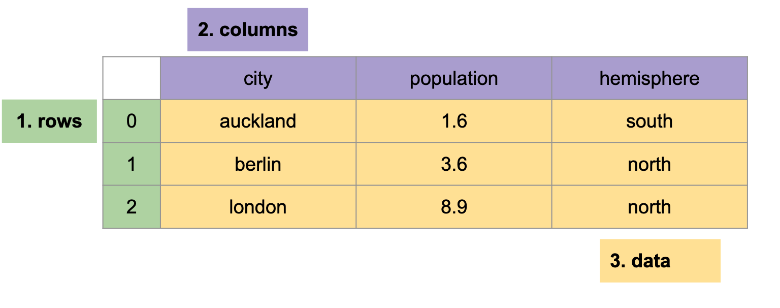
In this article we will work with a cities dataset - a tabular dataset with three rows and three columns:
Installing and Using Pandas
You can install pandas with pip, a Python package manager:
shell-session
$ pip install pandas
You can also find a notebook with all the code we develop in this article on Github or on Google Colab.
Pandas is used by importing the pandas package, commonly aliased to pd:
python
import pandas as pd
What is a DataFrame?
At the core of Pandas is the pd.DataFrame.
A pd.DataFrame has three parts:
- index - 1-dimensional row labels,
- columns - 1-dimensional column labels,
- values - 2-dimensional data.
The index and columns are labels - they tell us what a row or column represents, such as the population column label. The values are the data itself, like 1.6.
Creating a DataFrame
One way to create a DataFrame is from a Python dictionary, where the dictionary keys are the column names and the dictionary values are the data:
python
import pandas as pd

pd.DataFrame({
  'city': ['auckland', 'berlin', 'london'],
  'population': [1.6, 3.6, 8.9],
  'hemisphere': ['south', 'north', 'north']
})
"""
       city  population hemisphere
0  auckland         1.6      south
1    berlin         3.6      north
2    london         8.9      north
"""
Loading CSV Data into a DataFrame
Being able to construct DataFrames from Python objects such as dictionaries and lists is useful, but is limited to small datasets that we type manually in code. This is useful for creating data for unit tests, but not useful for working with large datasets.
A common way to create a DataFrame is from a CSV file. This allows us to work with CSV files on our local machine.
Pandas handles this with pd.read_csv, which reads data from a CSV file on our local computer.
This same function can also be used to read data from the Internet. Below we read in our cities dataset using pd.read_csv to read from a Github URI:
python
import pandas as pd

data = pd.read_csv(
    'https://raw.githubusercontent.com/ADGEfficiency/data-science-south-data/main/cities/cities.csv'
)
"""
       city  population hemisphere
0  auckland         1.6      south
1    berlin         3.6      north
2    london         8.9      north
"""
This is the way we will load our cities dataset in rest of this post - reading directly from a public URI (such as a URL).
Index, Columns & Values
We can access the three parts of our DataFrame as attributes of an initialized pd.Dataframe object:
python
data.index
# RangeIndex(start=0, stop=3, step=1)

data.columns
# Index(['city', 'population', 'hemisphere'], dtype='object')

data.values
"""
[['auckland' 1.6 'south']
 ['berlin' 3.6 'north']
 ['london' 8.9 'north']]
"""
The index pandas created for us is a range index (also called an integer index).
Rows are labelled with a sequence of integers ([0, 1, 2]):
python
data.index
# RangeIndex(start=0, stop=3, step=1)

data
"""
       city  population hemisphere
0  auckland         1.6      south
1    berlin         3.6      north
2    london         8.9      north
"""
We can replace this with more meaningful index using set_index, turning the city column into the index:
python
data.set_index('city')
"""
          population hemisphere
city
auckland         1.6      south
berlin           3.6      north
london           8.9      north
"""
We have lost our original integer index of [0, 1, 2] and gained an index of city - great!
Selecting Rows and Columns in Pandas
A basic operation in data analysis is selection - to select rows and columns. There are two ways to do this in pandas - loc and iloc.
Pandas offers two ways to do selection - one using a label and one using the integer position.
In Pandas we can select by a label using loc and by position using iloc. These two selection methods can be used on both the rows (index) and the columns of a DataFrame. We can use : to select the entire row or column.
loc Uses Labels
loc selects based on the label of the row and column.
loc allows us to use the labels of the index and columns - we use it to select data based on labels:
python
#  select the berlin row, all columns
data.loc['berlin', :]

#  select all rows, second column
data.loc[:, 'population']
iloc Uses Position
iloc selects based on the integer position of the row and column.
iloc allows us to use the position of rows and columns - we use it to select data based on position:
python
#  select the first row, all columns
data.iloc[0, :]

#  select all rows, second column
data.iloc[:, 1]
Selecting based on position is very useful when your data is sorted.
iloc is why a range index isn't that useful in pandas - we can always use iloc to select data based on it's position.
Now we have been introduced to loc & iloc, let's use them to answer two questions about our cities dataset.
What is the Population of Auckland?
We can answer this using loc, selecting the auckland row and the population column:
python
data.loc['auckland', 'population']
# 1.6
Which Hemisphere is our First City In?
We can answer this using iloc to select the first row with 0 and loc to select the population column:
python
data.iloc[0].loc['hemisphere']
# north
Filtering with Boolean Masks in Pandas
Another basic operation in data analysis is filtering - selecting rows or columns based on conditional logic (if statements, equalities like == and inequalities like > or <).
We can filter in pandas with a boolean mask, which can be created with a conditional statement:
python
import pandas as pd

data = pd.read_csv('https://raw.githubusercontent.com/ADGEfficiency/data-science-south-data/main/cities/cities.csv')

#  create our boolean mask
#  with the conditional 'population < 2.0'
#  aka population less than 2.0
mask = data.loc[:, 'population'] < 2.0
"""
city
auckland     True
berlin      False
london      False
Name: population, dtype: bool
"""
The boolean mask is an array of either True or False - here indicating True if the population of the city is less than 2.
We can use our boolean mask to filter our dataset with loc - loc understands how to use a boolean mask:
python
subset = data.loc[mask, :]
"""
          population hemisphere
city
auckland         1.6      south
"""
Why Do We Need Boolean Masks if We Can Select with loc or iloc?
The power of using boolean masks is that we can select many rows at once.
Below we create a boolean mask based on the hemisphere of the city - then using this mask to select two rows:
python
mask = data.loc[:, 'hemisphere'] == 'north'
"""
city
auckland    False
berlin       True
london       True
Name: hemisphere, dtype: bool
"""

subset = data.loc[mask, :]
"""
        population hemisphere
city
berlin         3.6      north
london         8.9      north
"""
Aggregation with Groupby in Pandas
The final data analysis operation we will look at is aggregation.
In Pandas aggregation can be done by grouping - using the groupby method on a DataFrame.
The Two Step Groupby Workflow
In Pandas aggregation happens in two steps:
- creating groups based on a column, such as by
hemisphere, - applying an aggregation function to each group, such as counting or averaging.
Aggregation allows us to estimate statistics, lets use it to answer a few more questions.
What is the Average Population In Each Hemisphere?
We can answer this with our two step workflow:
groupby('hemisphere')to group by hemisphere,mean()to calculate the average for each of our hemisphere groups (northandsouth).
python
import pandas as pd

data = pd.read_csv('https://raw.githubusercontent.com/ADGEfficiency/data-science-south-data/main/cities/cities.csv').set_index('city')
data.groupby('hemisphere').mean()
"""
            population
hemisphere
north             6.25
south             1.60
"""
What is the Total Population In Each Hemisphere?
Our two steps to answer this question are:
- grouping by
hemisphere, - aggregating with a
sum.
python
data.loc[:, ['population', 'hemisphere']].groupby('hemisphere').sum()
"""
            population
hemisphere
north             12.5
south              1.6
"""
Saving DaatFrame to CSV
The end of many data analysis pipelines involves saving data to disk - below we save our aggregation to a CSV file:
python
data.to_csv('groups.csv')
Full Pandas Code
All the code we looked at above is in full below:
python
#  import & alias pandas as pd
import pandas as pd

#  read dataset from github url
data = pd.read_csv('https://raw.githubusercontent.com/ADGEfficiency/data-science-south-data/main/cities/cities.csv').set_index('city')

#  save cities dataset to file on local machine
data.to_csv('cities.csv')

#  select the berlin row, all columns
data.loc['berlin', :]

#  select all rows, second colun
data.loc[:, 'population']

#  select the first row, all columns
data.iloc[0, :]

#  select all rows, second column
data.iloc[:, 1]

#  what is the population of Auckland?
data.loc['auckland', 'population']

#  which hemisphere is our first city in?
data.iloc[0].loc['hemisphere']

#  select population less than 2
subset = data.loc[data.loc[:, 'population'] < 2.0, :]

#  northern hemisphere countries
subset = data.loc[data.loc[:, 'hemisphere'] == 'north', :]

#  average population in each hemisphere
data.groupby('hemisphere').mean()

#  total population in each hemisphere
data.loc[:, ['population', 'hemisphere']].groupby('hemisphere').sum()

#  save to csv file on local computer
data.to_csv('groups.csv')
Matplotlib
Matplotlib is a Python library for creating data visualizations.
One challenge of Matplotlib is that it offers multiple ways to plot data. This means that there are different ways to do the same thing in Matplotlib. This can make using Matplotlib challenging as it's not clear which API is being used.
Mastering Matplotlib requires understanding the different Matplotlib APIs, and using whichever is best for your data and workflow.
We recommend and will use the plt.subplots API. It offers the flexibility to plot multiple charts in the same figure, and integrates nicely with Pandas.
Installing and Using Matplotlib
You can install Matplotlib with pip:
shell-session
$ pip install matplotlib
Matplotlib is used in Python by importing the matplotlib package, commonly aliasing the submodule matplotlib.pyplot as plt:
python
import matplotlib.pyplot as plt
What is a Matplotlib Figure?
The core components in Matplotlib are the figure and axes.
An axes is a single plot within a figure. A figure can have ore or more axes. Each axes can be thought of as a separate plot.
This axes is different from an axis, such as the y-axis or x-axis of a plot. An axes will have both a y-axis and x-axis.
Using the plt.subplots Matplotlib API
We can create a figure with two axes with the plt.subplots API:
python
import matplotlib.pyplot as plt

fig, axes = plt.subplots(ncols=2)
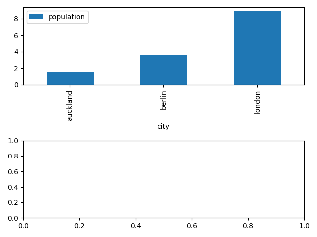
Our figure with two axes are at this point both empty.
Next we load our data with Pandas, and create a plot on our first axes:
python
import pandas as pd

#  load data from CSV with pandas
data = pd.read_csv('https://raw.githubusercontent.com/ADGEfficiency/data-science-south-data/main/cities/cities.csv').set_index('city')

#  create a bar plot on the first axes of our figure
data.plot('population', ax=axes[0], kind='bar')
Automatically makes labels for the x and y axis - quite nice!
Our second axes is still empty - we can plot something on it by passing ax=axes[1] into another plot call on our DataFrame:
python
#  access first axes and plot a scatter plot
data.plot('land-area', 'population', ax=axes[1], kind='scatter')
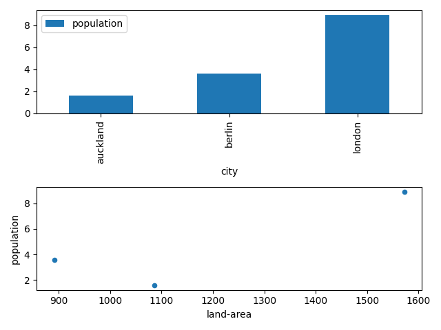
Now we can see two visualizations of our data - a bar chart and a scatter plot.
The final step in our pipeline is to save our figure to a PNG file on our local machine:
python
fig.savefig('cities.png')
Full Matplotlib Code
The full code for our visualization pipeline is below:
python
import matplotlib.pyplot as plt
import pandas as pd

#  create one figure with two axes
fig, axes = plt.subplots(nrows=2)

#  run a simple data pipeline
data = pd.read_csv('https://raw.githubusercontent.com/ADGEfficiency/data-science-south-data/main/cities/cities.csv').set_index('city')

#  access first axes and plot a line
data.plot(y='population', ax=axes[0], kind='bar')

#  access first axes and plot a scatter plot
data.plot('land-area', 'population', ax=axes[1], kind='scatter')

#  small trick to get x-axis labels to play nice
plt.tight_layout()

#  save the figure as a png file
fig.savefig('cities.png')
Summary
Thanks for reading!
Key takeaways from this post are:
- a
pd.DataFrameis made of an index, columns and values, .locselects based on the label,ilocselects based on position,- boolean masks can be used to select rows based on conditional logic,
- aggregation functions can be used with
.groupby, - the
plt.subplotsAPI is the best way to use Matplotlib.
This content is a sample from our Introduction to Pandas course.
Thanks for reading!
If you enjoyed this blog post, make sure to check out our free 77 data science lessons across 22 courses.